Tensor Simulation#
The tensor protocol lets you query the tensor (vector, matrix, etc.) representation of a bloq. For example, we can easily inspect the familiar unitary matrix representing the controlled-not operation:
from qualtran.bloqs.basic_gates import CNOT

cnot = CNOT()
cnot.tensor_contract().real
array([[1., 0., 0., 0.],
       [0., 1., 0., 0.],
       [0., 0., 0., 1.],
       [0., 0., 1., 0.]])
Bloqs can represent states, effects, unitary operations, and compositions of these operations. Below, we see the vector representation of the plus state and zero effect.
from qualtran.bloqs.basic_gates import PlusState, ZeroEffect

print('|+> \t', PlusState().tensor_contract())  # state
print('<0| \t', ZeroEffect().tensor_contract()) # effect
|+> 	 [0.70710678+0.j 0.70710678+0.j]
<0| 	 [1.+0.j 0.+0.j]
We can also look at the non-unitary And operation which outputs its result to a new qubit. As such, it’s shape is \((2^3, 2^2)\) instead of being a square matrix.
from qualtran.bloqs.mcmt import And

And().tensor_contract().shape
(8, 4)
For a bloq with exclusively thru-registers, the returned tensor will be a matrix with shape (n, n) where n is the number of bits in the signature. For a bloq with exlusively right- or left-registers, the returned tensor will be a vector with shape (n,). In general, the tensor will be an ndarray of shape (n_right_bits, n_left_bits); but empty dimensions are dropped.
Interface#
The main way of accessing the dense, contracted, tensor representation of a bloq or composite bloq is through the Bloq.tensor_contract() method as we’ve seen.
All functionality for the tensor protocol is contained in the qualtran.simulation.tensor module. For example: Bloq.tensor_contract() is an alias for bloq_to_dense(bloq: Bloq) within that module.
import numpy as np
from qualtran.simulation.tensor import bloq_to_dense

np.array_equal(
    cnot.tensor_contract(),
    bloq_to_dense(cnot)
)
True
Additional functionality#
Direct manipulation of the qtn.TensorNetwork#
A composite bloq can be easily transformed into a tensor network. We use Quimb to handle efficient contraction of such networks.
The most important library function is qualtran.simulation.tensor.cbloq_to_quimb. This will build a quimb qtn.TensorNetwork tensor network representation of the composite bloq. You may want to manipulate this object directly using the full Quimb API. Otherwise, this function is used as the workhorse behind the public functions and methods like Bloq.tensor_contract().
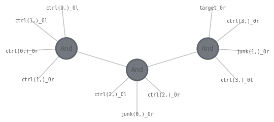
As an example below, we decompose MultiAnd into a CompositeBloq consisting of a ladder of two-bit Ands.
from qualtran.bloqs.mcmt import MultiAnd
from qualtran.drawing import show_bloq

bloq = MultiAnd(cvs=(1,)*4)
cbloq = bloq.decompose_bloq()
show_bloq(cbloq)

This composite bloq graph can be transformed into a quimb tensor network. Some of the visual flair has been lost, but the topology of the graph is the same.
from qualtran.simulation.tensor import cbloq_to_quimb

tn = cbloq_to_quimb(cbloq, friendly_indices=True)
tn.draw()
With this qtn.TensorNetwork in hand, the entire suite of Quimb tools are available.
tn.contraction_info()
  Complete contraction:  abcde,efghi,ijklm->abcdfghjklm
         Naive scaling:  13
     Optimized scaling:  12
      Naive FLOP count:  2.458e+4
  Optimized FLOP count:  9.216e+3
   Theoretical speedup:  2.667e+0
  Largest intermediate:  2.048e+3 elements
--------------------------------------------------------------------------------
scaling        BLAS                current                             remaining
--------------------------------------------------------------------------------
   9           GEMM  efghi,abcde->fghiabcd           ijklm,fghiabcd->abcdfghjklm
  12           TDOT fghiabcd,ijklm->abcdfghjklm         abcdfghjklm->abcdfghjklm
Quimb index format#
Above, we used the friendly_indices=True argument to give string names to the outer indices of the qtn.TensorNetwork. This can be useful for interactive manipulation of the tensor network by a human. Qualtran uses a highly-structured (but less human-readible) format for internal tensor indices, which we describe here.
In CompositeBloq, we form the compute graph by storing a list of nodes and edges. Quimb uses a different strategy for representing the tensor network graphs. To form a tensor network in Quimb, we provide a list of qtn.Tensor which contain not only the tensor data but also a list of “indices” that can form connections to other tensors. Similar to the Einstein summation convention, if two tensors each have an index with the same name: an edge is created in the tensor network graph and this shared index is summed over. In the Quimb documentation (for example), these indices are traditionally short strings like "k", but can be any hashable Python object. In CompositeBloq, the unique object that identifies a connection between bloqs is qualtran.Connection, so we use these connection objects as the first part of our indices.
Qualtran and Quimb both support “wires” with arbitrary bitsize. Qualtran uses bookkeeping bloqs like Join and Split to fuse and un-fuse indices. In theory, these operations should be free in the tensor contraction, as they are essentially an identity tensor. In our understanding, Quimb does not have special support for handling these re-shaping operations within the tensor network graph. In versions of Qualtran prior to v0.5, split and join operations were tensored up to n-sized identity tensors. This would form a bottleneck in any contraction ordering. Therefore, we keep all the indices un-fused in the tensor network representation and use tuples of (cxn, j) for our tensor indices, where the second integer j indexes the individual bits in a register with reg.dtype.num_bits > 1.
In summary:
Each tensor index is a tuple
(cxn, j)The
cxn: qualtran.Connectionentry identifies the connection between soquets in a Qualtran compute graph.The second integer
jis the bit index within high-bitsize registers, which is necessary due to technical restrictions.
example_inner_index = tn.inner_inds()[0]
cxn, j = example_inner_index
print("cxn:", cxn)
print("j:  ", j)
cxn: And<0>.target -> And<1>.ctrl[0]
j:   0
Flattening#
A call to Bloq.tensor_contract will first “flatten” the bloq by doing bloq.as_composite_bloq().flatten(). This is a sensible default default for constructing tensor networks, as the best contraction performance can generally be achieved by keeping tensors as small as possible in the network.
In Qualtran, we usually avoid flattening bloqs and strongly to prefer to work with one level of decomposition at a time. This is to avoid performance issues with large, abstract algorithms. But typically if the full circuit is large enough to cause performance issues with flattening it is also too large to simulate numerically; so an exception to the general advice is made here.
All bloqs in the flattened circuit must provide their explicit tensors. If your bloq’s tensors ought to be derived from its decomposition: this is achieved by the previously mentioned flattening operation. If a bloq provides tensors through overriding Bloq.my_tensors and also defines a decomposition, the explicit tensors will not be used (by default). If you’d like to always use annotated tensors, set bloq_to_dense(..., full_flatten=False). If you would like full control over flattening, use the free functions to control the tensor network construction and contraction.
# Set `full_flatten=False` to use annotated tensors even
# if there's a decomposition. (No change in this example since
# most bloqs don't define both a decomposition and tensors).
_ = bloq_to_dense(bloq, full_flatten=False)
# Manually flatten and contract for complete control
custom_flat = bloq.as_composite_bloq().flatten(lambda binst: binst.i != 2)
tn = cbloq_to_quimb(custom_flat)
len(tn.tensors)
3
Implementation#
The qualtran.simulation.tensor functions rely on the Bloq.my_tensors(...) method to implement the protocol. This is where a bloq’s tensor information is actually encoded.
Usually, the most efficient way of supporting tensor simulation is by providing a decomposition for your bloq. However, bloq authors may want to override my_tensors if the bloq can’t or shouldn’t define a decomposition. The method takes dictionaries of incoming and outgoing indices (keyed by register name) to asist the author in matching up dimensions of their np.ndarray to the incoming and outgoing wires when constructing qtn.Tensors.
The docstring for Bloq.my_tensors provides a complete, technical description of how to successfully override this method. In brief, the method must return one or more qtn.Tensors that get added to the tensor network. The indices used to construct these must be of the correct form. Each tensor index is a tuple (cxn, j). The connection entry comes from the incoming and outgoing arguments to the method. The j integer is the bit index within multi-bit registers.
New, we write our own CNOT bloq with custom tensors.
from functools import cached_property
from typing import Any, Dict, Tuple, List

import numpy as np
import quimb.tensor as qtn
from attrs import frozen

from qualtran import Bloq, Signature, Soquet, SoquetT, Register, Side

@frozen
class MyCNOT(Bloq):
    @cached_property
    def signature(self) -> 'Signature':
        return Signature.build(ctrl=1, target=1)

    def my_tensors(
        self, incoming: Dict[str, 'ConnectionT'], outgoing: Dict[str, 'ConnectionT']
    ) -> List['qtn.Tensor']:
        # The familiar CNOT matrix. We make sure to
        # cast this to np.complex128 so we don't accidentally
        # lose precision anywhere else in the contraction.
        matrix = np.array([
            [1, 0, 0, 0],
            [0, 1, 0, 0],
            [0, 0, 0, 1],
            [0, 0, 1, 0],
        ], dtype=np.complex128)

        # According to our signature, we have two thru-registers.
        # This means two incoming and two outgoing wires.
        # We'll reshape our matrix into the more natural n-dimensional
        # tensor form.
        tensor = matrix.reshape((2,2,2,2))

        # This is a simple case: we only need one tensor and
        # each register is one bit.
        outgoing_inds = [
            (outgoing['ctrl'], 0),
            (outgoing['target'], 0),
        ]
        incoming_inds = [
            (incoming['ctrl'], 0),
            (incoming['target'], 0),
        ]

        return [qtn.Tensor(
            data=tensor,
            inds=outgoing_inds + incoming_inds
        )]
# Sanity check
MyCNOT().tensor_contract()
array([[1.+0.j, 0.+0.j, 0.+0.j, 0.+0.j],
       [0.+0.j, 1.+0.j, 0.+0.j, 0.+0.j],
       [0.+0.j, 0.+0.j, 0.+0.j, 1.+0.j],
       [0.+0.j, 0.+0.j, 1.+0.j, 0.+0.j]])
Default Fallback#
By default, the flattening operation in a given tensor contraction should mean that only a finite number of small, target-gateset bloqs
should need to explicitly override my_tensors().
If a bloq does not override my_tensors(...) and doesn’t provide a decomposition, the tensor protocol will throw an error when trying to construct a tensor network.
For example, we author a BellState bloq. We define a decomposition but do not explicitly provide tensor information.
from qualtran import QBit
from qualtran.bloqs.basic_gates import PlusState, ZeroState

@frozen
class BellState(Bloq):
    @cached_property
    def signature(self) -> 'Signature':
        return Signature([
            Register('q0', QBit(), side=Side.RIGHT),
            Register('q1', QBit(), side=Side.RIGHT)
        ])

    def build_composite_bloq(self, bb):
        q0 = bb.add(PlusState())
        q1 = bb.add(ZeroState())

        q0, q1 = bb.add(CNOT(), ctrl=q0, target=q1)
        return {'q0': q0, 'q1': q1}
The system can still contract the tensor network implied by this bloq because it will automatically flatten the bloq.
print(BellState().tensor_contract())
[0.70710678+0.j 0. +0.j 0. +0.j 0.70710678+0.j]
If you try to directly use cbloq_to_quimb and bypass the flattening operation, an error will be raised.
try:
    cbloq_to_quimb(BellState().as_composite_bloq())
except NotImplementedError as e:
    print("Expected error because we didn't flatten first:", repr(e))
Expected error because we didn't flatten first: NotImplementedError('BellState does not support tensor simulation.')
Properties and Relations#
Gates with factorized tensors#
The my_tensors method can return multiple Tensor objects if there is a known factorization of the bloq’s tensors. For example: CNOT can be written as a dense 4x4 matrix or by contracting the so-called COPY and XOR tensors.
from qualtran.bloqs.basic_gates import CNOT
from qualtran.simulation.tensor import cbloq_to_quimb

cbloq = CNOT().as_composite_bloq()
tn = cbloq_to_quimb(cbloq, friendly_indices=True)

tn.draw(color=['COPY', 'XOR'], show_tags=True, initial_layout='spectral')
for tensor in tn:
    print(tensor.tags)
    print(tensor.data)
    print()

oset(['COPY'])
[[[1.+0.j 0.+0.j]
  [0.+0.j 0.+0.j]]

 [[0.+0.j 0.+0.j]
  [0.+0.j 1.+0.j]]]

oset(['XOR'])
[[[1.+0.j 0.+0.j]
  [0.+0.j 1.+0.j]]

 [[0.+0.j 1.+0.j]
  [1.+0.j 0.+0.j]]]
Final state vector from a circuit#
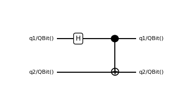
In Qualtran, all initial states must be explicitly specified with allocation-like bloqs. For example, if we define the circuit below, the .tensor_contract simulation method will only ever return a unitary matrix. If you’d like the state vector that results from applying that circuit to qubits initialized in a particular way (e.g. the all-zeros computational basis state), then you must specify that
from qualtran import BloqBuilder
from qualtran.bloqs.basic_gates import Hadamard

bb = BloqBuilder()
q1 = bb.add_register('q1', 1)
q2 = bb.add_register('q2', 1)

q1 = bb.add(Hadamard(), q=q1)
q1, q2 = bb.add(CNOT(), ctrl=q1, target=q2)
bell_circuit = bb.finalize(q1=q1, q2=q2)

# This circuit always corresponds to a unitary *matrix*
show_bloq(bell_circuit, 'musical_score')
print(bell_circuit.tensor_contract().round(2))
[[ 0.71+0.j  0.  +0.j  0.71+0.j  0.  +0.j]
 [ 0.  +0.j  0.71+0.j  0.  +0.j  0.71+0.j]
 [ 0.  +0.j  0.71+0.j  0.  +0.j -0.71+0.j]
 [ 0.71+0.j  0.  +0.j -0.71+0.j  0.  +0.j]]
We can use the initialize_from_zero helper function to get the state vector corresponding to an all-zeros initial state.
from qualtran.simulation.tensor import initialize_from_zero
bell_state_cbloq = initialize_from_zero(bell_circuit)

# The new composite bloq consists of a round of intialization and
# then the circuit from above. Its tensor contraction is the state vector
show_bloq(bell_state_cbloq)
print(bell_state_cbloq.tensor_contract().round(2))

[0.71+0.j 0. +0.j 0. +0.j 0.71+0.j]