Quantum Variable Rotation

Quantum variable rotation (QVR) represents a family of Bloqs that can act as a Phase Oracle[1, 2], i.e. it implements a unitary which phases each computational basis state \(|x\rangle\), on which the wave-function has support, by an amount \(e^{i 2\pi \gamma x}\). The general unitary can be defined as

\[ \text{QVR}_{n, \epsilon}(\gamma)\sum_{j=0}^{2^n-1} c_j|x_j\rangle\rightarrow\sum_{j=0}^{2^n-1} e^{2\pi i\widetilde{\gamma x_j}}c_j|x_j\rangle \]

where \(\epsilon\) parameterizes the accuracy to which we wish to synthesize the phase coefficients s.t.

\[ |e^{2\pi i\widetilde{\gamma x_j}} - e^{2\pi i \gamma x_j}| \leq \epsilon \]

which, using rules of propagation of error [3], implies

\[ |\gamma x_j - \widetilde{\gamma x_j}| \leq \frac{\epsilon}{2\pi} \]

The linked references typically assume that \(0 \leq x_{j} \le 1\) and \(-1 \leq \gamma \leq 1\), for ease of exposition and analysis, but we do not have any such constraint. In the implementations presented below, both the cost register \(|x\rangle\) and \(\gamma\) can be arbitrary fixed point integer types. Each section below presents more details about the constraints on cost register \(|x\rangle\) and scaling constant \(\gamma\).

References:

1. Faster quantum chemistry simulation on fault-tolerant quantum computers Fig 14.

2. Compilation of Fault-Tolerant Quantum Heuristics for Combinatorial Optimization Appendix C: Oracles for phasing by cost function

3. Formulae for propagating uncertainty

from qualtran import Bloq, CompositeBloq, BloqBuilder, Signature, Register
from qualtran import QBit, QInt, QUInt, QAny
from qualtran.drawing import show_bloq, show_call_graph, show_counts_sigma
from typing import *
import numpy as np
import sympy
import cirq

QvrZPow

QVR oracle that applies a ZPow rotation to every qubit in the n-bit cost register.

This phase oracle simply applies a \(Z^{2^{k}}\) rotation to every qubit in the cost register. To obtain a desired accuracy of \(\epsilon\), each individual rotation is synthesized with accuracy \(\frac{\epsilon}{n}\), where \(n\) is the size of cost register.

The toffoli cost of this method scales as

\[ \text{T-Cost} \approxeq \mathcal{O}\left(n \log{\frac{n}{\epsilon}} \right) \]

Note that when \(n\) is large, we can ignore small angle rotations s.t. number of rotations to synthesize \(\leq \log{\left(\frac{2\pi \gamma}{\epsilon}\right)}\)

Thus, the T-cost scales as

\[\begin{split}\begin{aligned} \text{T-Cost} &\approxeq \mathcal{O}\left(n \log{\frac{n}{\epsilon}} \right) \\ &\approxeq \mathcal{O}\left(\log^2{\frac{1}{\epsilon}} + \log{\left(\frac{1}{\epsilon}\right)} \log{\left(\log{\left(\frac{1}{\epsilon}\right)}\right)}\right) \end{aligned}\end{split}\]

Parameters

• cost_reg: Cost register of dtype QFxp. Supports arbitrary QFxp types, including signed and unsigned.

• gamma: Scaling factor to multiply the cost register by, before applying the phase. Can be arbitrary floating point number.

• eps: Precision for synthesizing the phases.

from qualtran.bloqs.rotations import QvrZPow

Example Instances

qvr_zpow = QvrZPow.from_bitsize(12, gamma=0.1, eps=1e-2)

Graphical Signature

from qualtran.drawing import show_bloqs
show_bloqs([qvr_zpow],
           ['`qvr_zpow`'])

Call Graph

from qualtran.resource_counting.generalizers import ignore_split_join
qvr_zpow_g, qvr_zpow_sigma = qvr_zpow.call_graph(max_depth=1, generalizer=ignore_split_join)
show_call_graph(qvr_zpow_g)
show_counts_sigma(qvr_zpow_sigma)

Counts totals:

• Z**0.0015625: 6

QvrPhaseGradient

QVR oracle that applies a rotation via addition into the phase gradient register.

A \(b_\text{grad}\)-bit phase gradient state \(|\phi\rangle_{b_\text{grad}}\) can be written as

\[\begin{split} \begin{aligned} |\phi\rangle_{b_\text{grad}} &= \frac{1}{\sqrt{2^{b_\text{grad}}}} \sum_{k=0}^{2^{b_\text{grad}} - 1} e^{\frac{-2\pi i k}{2^{b_\text{grad}}}} |\frac{k}{2^{b_\text{grad}}}\rangle \\ &= \text{QVR}_{(b_\text{grad}, b_\text{grad}), \epsilon}(-1) |+\rangle ^ {b_\text{grad}} \end{aligned} \end{split}\]

In the above equation \(\frac{k}{2^{b_\text{grad}}}\) represents a fixed point fraction. In Qualtran, we can represent such a quantum register using quantum data type QFxp(bitsize=b_grad, num_frac=b_grad, signed=False). Let \(\tilde{k}=\frac{k}{2^{b_\text{grad}}}\) be a \(b_\text{grad}\)-bit fixed point fraction, we can rewrite the phase gradient state as

\[ |\phi\rangle_{b_\text{grad}} = \frac{1}{\sqrt{2^{b_\text{grad}}}} \sum_{\tilde{k}=0}^{\frac{2^{b_\text{grad}}-1}{2^{b_\text{grad}}}} e^{-2\pi i \tilde{k}} \ket{\tilde{k}} \]

A useful property of the phase gradient state is that adding a fixed-point number \(\tilde{l}\) to the state applies a phase-kickback of \(e^{2\pi i \tilde{l}}\)

\[ |\phi + \tilde{l}\rangle_{b_\text{grad}} = e^{2\pi i \tilde{l}}|\phi\rangle_{b_\text{grad}} \]

We exploit this property of the phase gradient states to implement a quantum variable rotation via addition into the phase gradient state s.t.

\[\begin{split}\begin{aligned} \text{QVR}_{n,\epsilon}(\gamma)|x\rangle|\phi\rangle &=|x\rangle|\phi+\gamma x\rangle \\ &= e^{2\pi i \gamma x}|x\rangle |\phi\rangle \end{aligned}\end{split}\]

A number of subtleties arise as part of this procedure and we describe them below one by one.

• Adding a scaled value into phase gradient register Instead of computing \(\gamma x\) an intermediate register, we perform the multiplication via repeated additions into the phase gradient register, as described in [2]. This requires us to represent \(\gamma\) as a fixed point fraction with bitsize \(\gamma_\text{bitsize}\). This procedure introduces two sources of errors:

  • Errors due to fixed point representation of \(\gamma\) - Note that adding any fixed point number of the form \(a.b\) to the phase gradient register is equivalent to adding \(0.b\) since \(e^{2\pi i a} = 1\) for every integer \(a\). Let \(\tilde{\gamma} = a.b\) and \(x = p.q\) be fixed point decimal representations of \(\gamma\) and \(x\). We can write the product \(\gamma x\) as

    \[ \tilde{\gamma} x = (\sum_{i=0}^{\gamma_\text{n\_int}} a_{i} * 2^{i} + \sum_{i=1}^{\gamma_\text{n\_frac}} \frac{b_i}{2^i}) (\sum_{j=0}^{x_\text{n\_int}} p_{j} * 2^{j} + \sum_{j=1}^{x_\text{n\_frac}} \frac{q_{j}}{2^{j}}) \]
    In order to compute \(\tilde{\gamma} x\) to precision \(\frac{\epsilon}{2\pi}\), we can ignore all terms in the above summation that are < \(\frac{\epsilon}{2\pi}\). Let \(b_\text{phase} = \log_2{\frac{2\pi}{\epsilon}}\), then we get \(\gamma_\text{n\_frac} = x_\text{n\_int} + b_\text{phase}\). Thus,

  \[\begin{split}\begin{aligned} \gamma_\text{bitsize} &= \gamma_\text{n\_int} + x_\text{n\_int} + b_\text{phase} \\ &\approxeq \log_2{\frac{1}{\epsilon}} + x_\text{n\_int} + O(1) \end{aligned}\end{split}\]

  • Errors due to truncation of digits of \(|x\rangle\) during multiplication via repeated addition - Let \(b_\text{grad}\) be the size of the phase gradient register. When adding left/right shifted copies of state \(x\) to the phase gradient register, we incur an error every time the fractional part of the shifted state to be added needs to be truncated to \(b_\text{grad}\) digits. For each such addition the error is upper bounded by \(\frac{2\pi}{2^{b_\text{grad}}}\), because we omit adding bits that would correspond to phase shifts of \(\frac{2\pi}{2^{b_\text{grad}+1}}\), \(\frac{2\pi}{2^{b_\text{grad}+2}}\), and so forth. The number of such additions can be upper bounded by \(\frac{(\gamma_\text{bitsize} + 2)}{2}\) using techniques from [2].

    • When \(b_\text{grad} \geq x_\text{bitsize}\): the first \(x_\text{n\_int}\) additions do not contribute to any phase error and thus the number of error causing additions can be upper bounded by \(\frac{(b_\text{phase} + 2)}{2}\). In order to keep the error less than \(\epsilon\), we get

      \[\begin{split}\begin{aligned} b_\text{grad}&=\left\lceil\log_2{\frac{\text{num\_additions}\times2\pi}{\epsilon}} \right\rceil \\ &=\left\lceil\log_2{\frac{(b_\text{phase}+2)\pi}{\epsilon}}\right\rceil \text{; if } b_\text{grad} \geq x_\text{bitsize} \\ \end{aligned}\end{split}\]

    • When \(b_\text{grad} \lt x_\text{bitsize}\): We believe that the above precision for \(b_\text{grad}\) holds even for this case we have some numerics in tests to verify that. Currently, QvrPhaseGradient always sets the bitsize of phase gradient register as per the above equation.

• Constraints on \(\gamma\) and \(|x\rangle\) - In the current implementation, \(\gamma\) can be any arbitrary floating point number (signed or unsigned) and \(|x\rangle\) must be an unsigned fixed point register.

• Cost of the phase gradient procedure - Each addition into the phase gradient register costs \(b_\text{grad} - 2\) Toffoli’s and there are \(\frac{\gamma_\text{bitsize} + 2}{2}\) such additions, therefore the total Toffoli cost is

  \[\begin{split}\begin{aligned} \text{T-Cost} &= \frac{(b_\text{grad} - 2)(\gamma_\text{bitsize} + 2)}{2} \\ &\approxeq \mathcal{O}\left(\log^2{\frac{1}{\epsilon}} + \log{\left(\frac{1}{\epsilon}\right)} \log{\left(\log{\left(\frac{1}{\epsilon}\right)}\right)}\right) \end{aligned}\end{split}\]

Thus, for cases where \(-1\lt \gamma \lt 1\) and \(0 \leq x \lt 1\), the toffoli cost scales as \(\mathcal{O}\left(\log^2{\frac{1}{\epsilon}} \log{\log{\frac{1}{\epsilon}}}\right)\)

References

• Compilation of Fault-Tolerant Quantum Heuristics for Combinatorial Optimization. Section II-C: Oracles for phasing by cost function. Appendix A: Addition for controlled rotations

from qualtran.bloqs.rotations import QvrPhaseGradient

Example Instances

qvr_phase_gradient = QvrPhaseGradient.from_bitsize(12, gamma=0.1, eps=1e-4)

Graphical Signature

from qualtran.drawing import show_bloqs
show_bloqs([qvr_phase_gradient],
           ['`qvr_phase_gradient`'])

Call Graph

from qualtran.resource_counting.generalizers import ignore_split_join
qvr_phase_gradient_g, qvr_phase_gradient_sigma = qvr_phase_gradient.call_graph(max_depth=1, generalizer=ignore_split_join)
show_call_graph(qvr_phase_gradient_g)
show_counts_sigma(qvr_phase_gradient_sigma)

Counts totals:

• AddScaledValIntoPhaseReg: 1

QVR Cost analysis

T-Count Expression for QvrZpow

from qualtran.cirq_interop.t_complexity_protocol import TComplexity

def get_t_counts_qvr_zpow(n, gamma, eps):
    _, sigma = QvrZPow.from_bitsize(n, gamma, eps).call_graph()
    (bloq, counts), = [*sigma.items()]
    return TComplexity.rotation_cost(bloq.eps) * counts


get_t_counts_qvr_zpow(*sympy.symbols('n, \gamma, \epsilon'))

\[\displaystyle \left\lceil{1.149 \operatorname{log}_{2}{\left(\frac{1.0 \min\left(n, \left\lceil{\operatorname{log}_{2}{\left(\frac{2 \pi \left|{\gamma}\right|}{\epsilon} \right)}}\right\rceil\right)}{\epsilon} \right)} + 9.2}\right\rceil \min\left(n, \left\lceil{\operatorname{log}_{2}{\left(\frac{2 \pi \left|{\gamma}\right|}{\epsilon} \right)}}\right\rceil\right)\]

T-Count Expression for QvrPhaseGradient

from qualtran.resource_counting.t_counts_from_sigma import t_counts_from_sigma

def get_t_counts_qvr_phase_gradient(n, gamma, eps):
    _, sigma = QvrPhaseGradient.from_bitsize(n, gamma, eps).call_graph()
    return t_counts_from_sigma(sigma)


get_t_counts_qvr_phase_gradient(*sympy.symbols('n, \gamma, \epsilon'))

\[\displaystyle 4 \left(\left\lceil{\operatorname{log}_{2}{\left(\frac{\pi \left(2 \left\lfloor{\frac{\left\lceil{\operatorname{log}_{2}{\left(\frac{2 \pi}{\epsilon} \right)}}\right\rceil}{2}}\right\rfloor + 2\right)}{\epsilon} \right)}}\right\rceil - 2\right) \left(\left\lfloor{\frac{\left\lceil{\operatorname{log}_{2}{\left(\frac{2 \pi}{\epsilon} \right)}}\right\rceil}{2} + \frac{\max\left(0, \left\lceil{\operatorname{log}_{2}{\left(\left\lfloor{\left|{\gamma}\right|}\right\rfloor + 1 \right)}}\right\rceil\right)}{2}}\right\rfloor + 1\right)\]

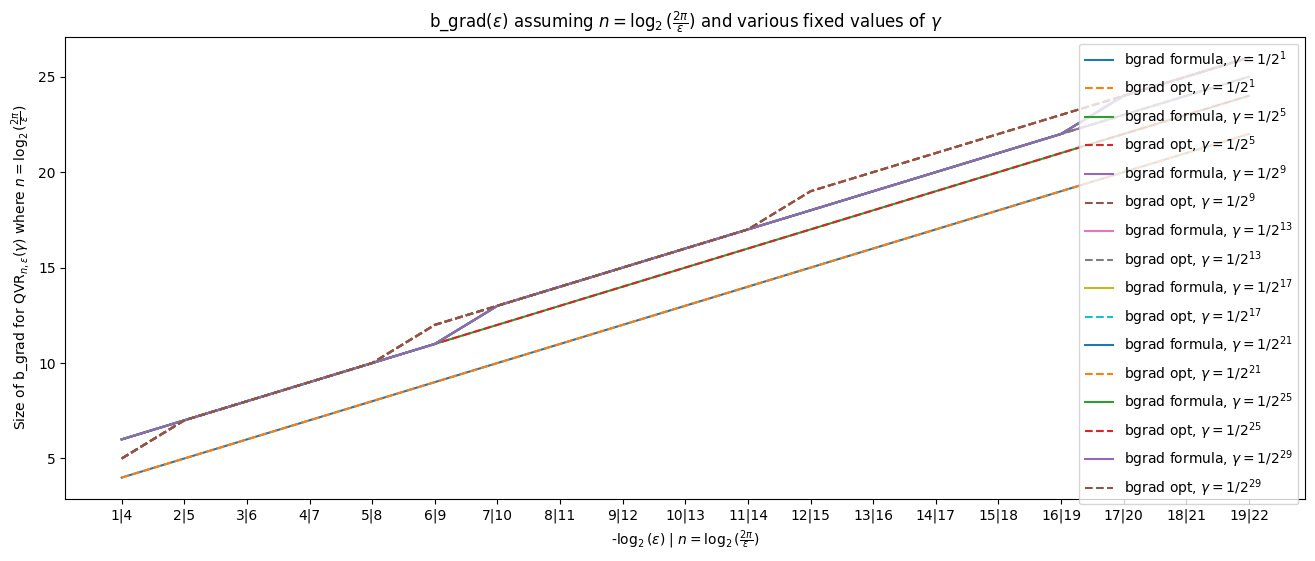
b_grad(\(\epsilon\)) assuming \(n=\log_2(\frac{2\pi}{\epsilon})\) and various fixed values of \(\gamma\)

import matplotlib.pyplot as plt

num_eps = 20
eps_vals = [1/2**i for i in range(1, num_eps)]
n_vals = [int(np.ceil(np.log2(2 * np.pi / eps))) for eps in eps_vals]
x_vals = [i for i in range(1, num_eps)]

bgrad_formula, bgrad_opt = [], []
gamma_ones = [i for i in range(1, 30, 4)]
for n_ones in gamma_ones:
    gamma = (2**n_ones - 1)/2**n_ones
    curr_formula, curr_opt = [], []
    for n, eps in zip(n_vals, eps_vals):
        bloq = QvrPhaseGradient.from_bitsize(n, gamma, eps)
        curr_formula.append(bloq.b_grad_via_formula)
        curr_opt.append(bloq.b_grad_via_fxp_optimization)
    bgrad_formula.append(tuple(curr_formula))
    bgrad_opt.append(tuple(curr_opt))


plt.figure(figsize=(16,6))
for i, n_ones in enumerate(gamma_ones):
    gamma_str = f"1/2^{{{n_ones}}}"
    plt.plot(x_vals, bgrad_formula[i], label=f'bgrad formula, $\gamma={gamma_str}$')
    plt.plot(x_vals, bgrad_opt[i], label=f'bgrad opt, $\gamma={gamma_str}$', linestyle='--')

x_labels = [f'{x}|{n}' for x, n in  zip(x_vals, n_vals)]
plt.xticks(ticks=x_vals, labels=x_labels)
plt.title(r'b_grad($\epsilon$) assuming $n=\log_2(\frac{2\pi}{\epsilon})$ and various fixed values of $\gamma$')
plt.ylabel(r'Size of b_grad for $\text{QVR}_{n, \epsilon}(\gamma)$ where $n=\log_2(\frac{2\pi}{\epsilon})$')
plt.xlabel(r'-$\log_{2}(\epsilon)$ | $n=\log_2(\frac{2\pi}{\epsilon})$')
plt.legend()

<matplotlib.legend.Legend at 0x7fde77f97450>

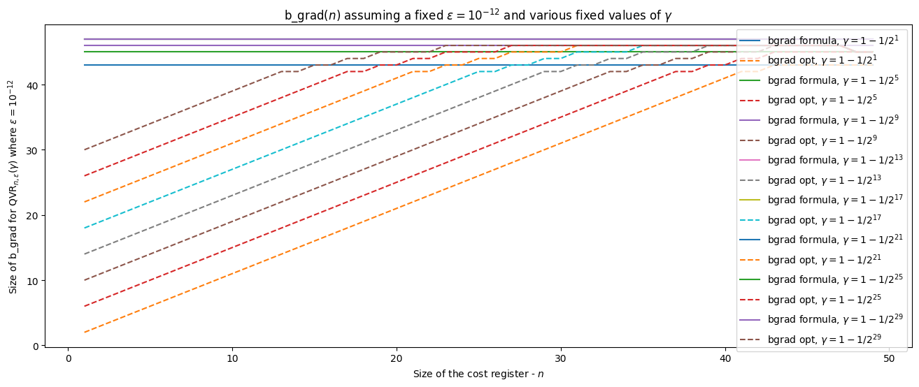
b_grad(\(n\)) assuming a fixed \(\epsilon = 10^{-12}\) and various fixed values of \(\gamma\)

import matplotlib.pyplot as plt

eps = 1e-12
n_vals = [*range(1, 50)]

x_vals = [n for n in n_vals]
bgrad_formula, bgrad_opt = [], []
gamma_ones = [i for i in range(1, 30, 4)]
for n_ones in gamma_ones:
    gamma = (2**n_ones - 1)/2**n_ones
    curr_formula, curr_opt = [], []
    for n in n_vals:
        bloq = QvrPhaseGradient.from_bitsize(n, gamma, eps)
        curr_formula.append(bloq.b_grad_via_formula)
        curr_opt.append(bloq.b_grad_via_fxp_optimization)
    bgrad_formula.append(tuple(curr_formula))
    bgrad_opt.append(tuple(curr_opt))


plt.figure(figsize=(16,6))
for i, n_ones in enumerate(gamma_ones):
    gamma_str = f"1 - 1/2^{{{n_ones}}}"
    plt.plot(x_vals, bgrad_formula[i], label=f'bgrad formula, $\gamma={gamma_str}$')
    plt.plot(x_vals, bgrad_opt[i], label=f'bgrad opt, $\gamma={gamma_str}$', linestyle='--')

plt.title(r'b_grad($n$) assuming a fixed $\epsilon = 10^{-12}$ and various fixed values of $\gamma$')
plt.ylabel(r'Size of b_grad for $\text{QVR}_{n, \epsilon}(\gamma)$ where $\epsilon=10^{-12}$')
plt.xlabel(r'Size of the cost register - $n$')
plt.legend()

<matplotlib.legend.Legend at 0x7fde6ad1f450>

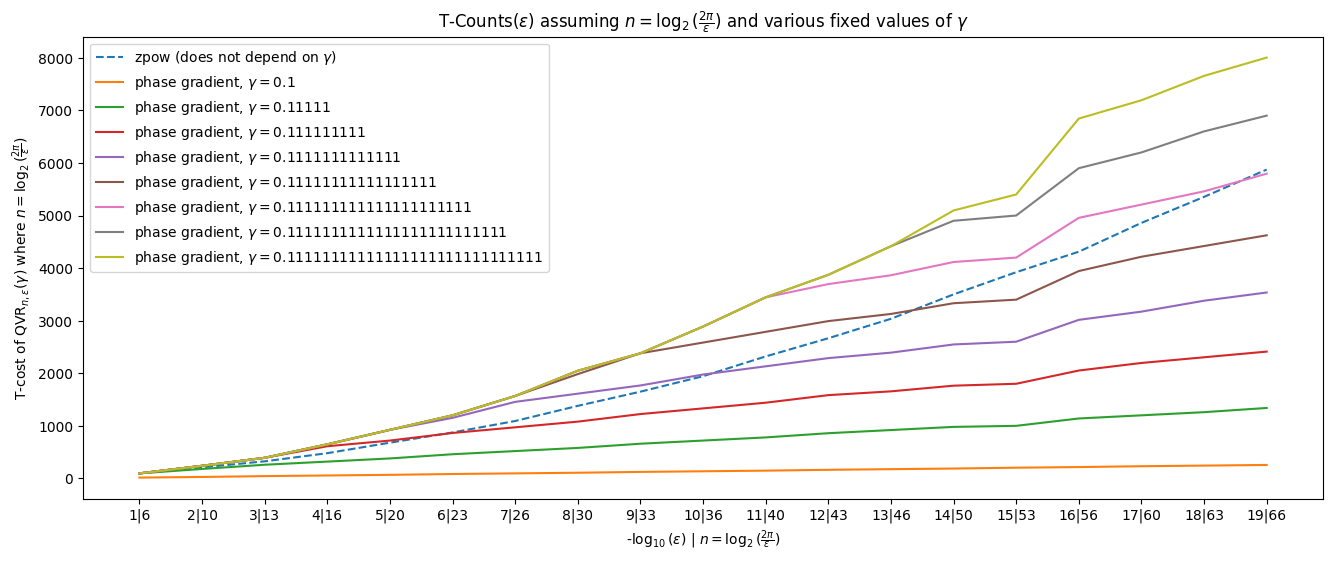
T-Counts(\(\epsilon\)) assuming \(n=\log_2(\frac{2\pi}{\epsilon})\) and various fixed values of \(\gamma\)

import matplotlib.pyplot as plt

num_eps = 20
x_vals = [i for i in range(1, num_eps)]
eps_vals = [1/10**i for i in range(1, num_eps)]
n_vals = [int(np.ceil(np.log2(2 * np.pi / eps))) for eps in eps_vals]
zpow_vals = [get_t_counts_qvr_zpow(n, 1, eps) for n, eps in zip(n_vals, eps_vals)]

pg = []
gamma_ones = [i for i in range(1, 30, 4)]
for n_ones in gamma_ones:
    gamma = (2**n_ones - 1)/2**n_ones
    pg.append([get_t_counts_qvr_phase_gradient(n, gamma, eps) for n, eps in zip(n_vals, eps_vals)])


plt.figure(figsize=(16,6))
plt.plot(x_vals, zpow_vals, label=r'zpow (does not depend on $\gamma$)', linestyle='--')
for i, n_ones in enumerate(gamma_ones):
    plt.plot(x_vals, pg[i], label=f'phase gradient, $\gamma=0.{"1"*n_ones}$')

x_labels = [f'{x}|{n}' for x, n in  zip(x_vals, n_vals)]
plt.xticks(ticks=x_vals, labels=x_labels)
plt.title(r'T-Counts($\epsilon$) assuming $n=\log_2(\frac{2\pi}{\epsilon})$ and various fixed values of $\gamma$')
plt.ylabel(r'T-cost of $\text{QVR}_{n, \epsilon}(\gamma)$ where $n=\log_2(\frac{2\pi}{\epsilon})$')
plt.xlabel(r'-$\log_{10}(\epsilon)$ | $n=\log_2(\frac{2\pi}{\epsilon})$')
plt.legend()

<matplotlib.legend.Legend at 0x7fde6d757450>

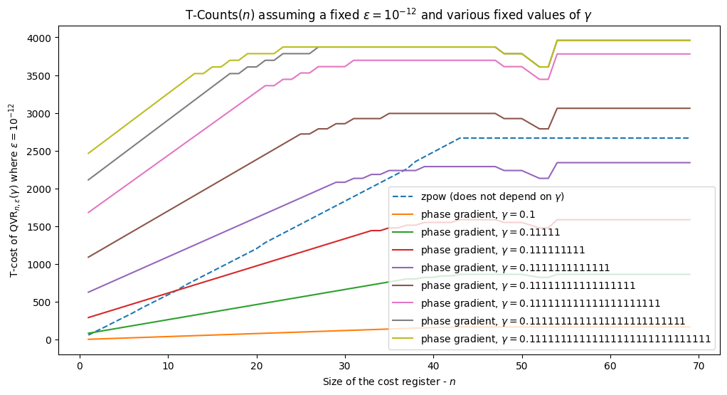
T-Counts(\(n\)) assuming a fixed \(\epsilon = 10^{-12}\) and various fixed values of \(\gamma\)

import matplotlib.pyplot as plt

eps = 1e-12
n_vals = [*range(1, 70)]

zpow_vals = [get_t_counts_qvr_zpow(n, 1, eps) for n in n_vals]

pg = []
for n_ones in gamma_ones:
    gamma = (2**n_ones - 1)/2**n_ones
    pg.append([get_t_counts_qvr_phase_gradient(n, gamma, eps) for n in n_vals])

plt.figure(figsize=(12,6))

x_vals = [n for n in n_vals]
plt.plot(x_vals, zpow_vals, label=r'zpow (does not depend on $\gamma$)', linestyle='--')
for i, n_ones in enumerate(gamma_ones):
    plt.plot(x_vals, pg[i], label=f'phase gradient, $\gamma=0.{"1"*n_ones}$')
plt.title(r'T-Counts($n$) assuming a fixed $\epsilon = 10^{-12}$ and various fixed values of $\gamma$')
plt.ylabel(r'T-cost of $\text{QVR}_{n, \epsilon}(\gamma)$ where $\epsilon=10^{-12}$')
plt.xlabel(r'Size of the cost register - $n$')
plt.legend()

<matplotlib.legend.Legend at 0x7fde63907ad0>